Quickstart

This public site can show how to use OptiXDE without exposing the private repository.

Installation

If OptiXDE is private, keep installation instructions generic:

# Option A: internal/private install (example)
pip install optixde --extra-index-url <YOUR_PRIVATE_INDEX>

# Option B: request access to the private repo
# (See the "Cite & Contact" page)

Install the public release

Public releases of OptiXDE can be installed directly from PyPI. The core package only requires NumPy; install optional features when they are needed.

pip install optixde

# Optional features
pip install "optixde[plot]"    # Matplotlib plotting helpers
pip install "optixde[sparse]"  # SciPy-based embedded-domain solvers
pip install "optixde[gpu]"     # PyTorch backend for GPU FFT solvers

Verify the installation by printing the installed version:

import optixde

print(optixde.__version__)

Geometry Construction Tutorial

OptiXDE runs on an FFT-compatible uniform grid, so geometry is represented implicitly as a mask field on that grid (not a mesh). The recommended public-facing pipeline is:

primitives → CSG → binary mask → smoothed mask → embedded/penalized PDE

This keeps the API simple while allowing complex shapes, and it’s safe to share publicly because it demonstrates usage rather than implementation.

---

1) Create a geometry (primitives)

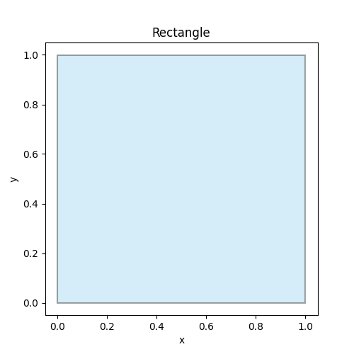
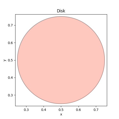
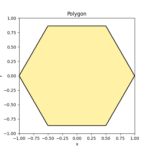
OptiXDE provides simple 2D primitives that can be composed later with CSG operations. Here are three basic examples.

Example 1: Rectangle

from optixde.geometry.primitives import Rectangle
from optixde.post.plotting import show_geometry

geo = Rectangle(0.0, 1.0, 0.0, 1.0)
show_geometry(geo, title="Rectangle", facecolor="skyblue", edgecolor="black")

Example 2: Disk

from optixde.geometry.primitives import Disk
from optixde.post.plotting import show_geometry

geo = Disk((0.5, 0.5), 0.25)
show_geometry(geo, title="Disk", facecolor="tomato", edgecolor="black")

Example 3: Polygon

from optixde.geometry.primitives import Polygon
from optixde.post.plotting import show_geometry

geo = Polygon([
    (1.0, 0.0),
    (0.5, 0.8660254),
    (-0.5, 0.8660254),
    (-1.0, 0.0),
    (-0.5, -0.8660254),
    (0.5, -0.8660254),
])
show_geometry(geo, title="Polygon", facecolor="gold", edgecolor="black")

2) Apply boolean operations

Boolean operations combine simple primitives into more complex shapes. In OptiXDE, the most common operations are:

• : union
• : intersection
• : difference

Below are three minimal examples using Rectangle, Disk, and Polygon.

---

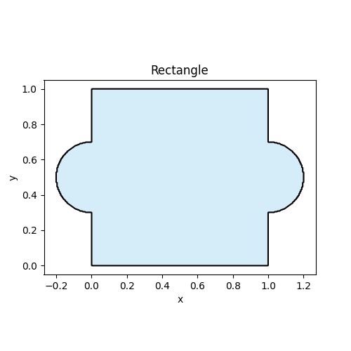
Example 1: Union of a rectangle and two circle

from optixde.geometry.primitives import Rectangle, Disk
from optixde.post.plotting import show_geometry
from optixde.geometry.boolean import Union

rect = Rectangle(0.0, 1.0, 0.0, 1.0)
left_circle  = Disk((0.0, 0.5), 0.2)
right_circle = Disk((1.0, 0.5), 0.2)
geo = Union(rect, left_circle, right_circle)
show_geometry(geo, title="Rectangle", facecolor="skyblue", edgecolor="black")

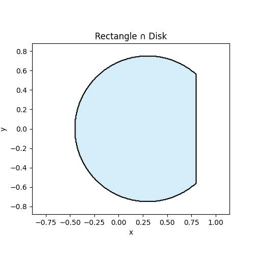
Example: Intersection of a rectangle and a disk

from optixde.geometry.primitives import Rectangle, Disk
from optixde.geometry.boolean import Intersection
from optixde.post.plotting import show_geometry

rect = Rectangle(-0.8, 0.8, -0.8, 0.8)
disk = Disk((0.3, 0.0), 0.75)

geo = Intersection(rect, disk)

show_geometry(
    geo,
    title="Rectangle ∩ Disk",
    facecolor="skyblue",
    edgecolor="black",
)

Example: Difference of a rectangle and a disk

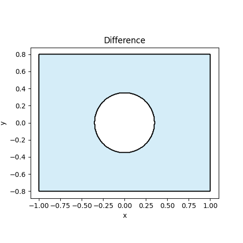
from optixde.geometry.primitives import Rectangle, Disk
from optixde.geometry.boolean import Difference
from optixde.post.plotting import show_geometry

rect = Rectangle(-1.0, 1.0, -0.8, 0.8)
hole = Disk((0.0, 0.0), 0.35)

geo = Difference(rect, hole)

show_geometry(
    geo,
    title="Difference",
    facecolor="skyblue",
    edgecolor="black",
)

3) From geometry to mask field

OptiXDE represents geometry on an FFT-compatible uniform grid as a mask field.

Example: geometry to binary mask

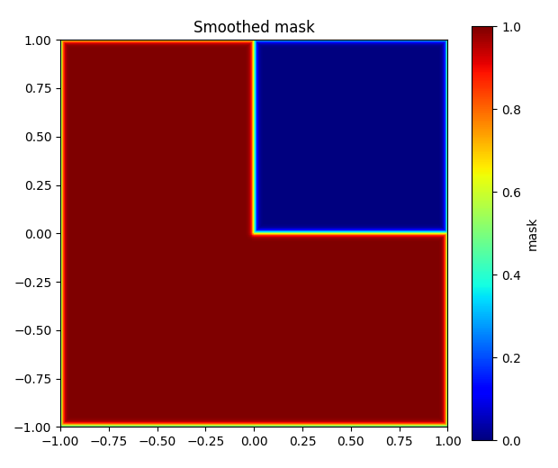
The geometry can be sampled on a uniform Cartesian grid and represented as a mask field.
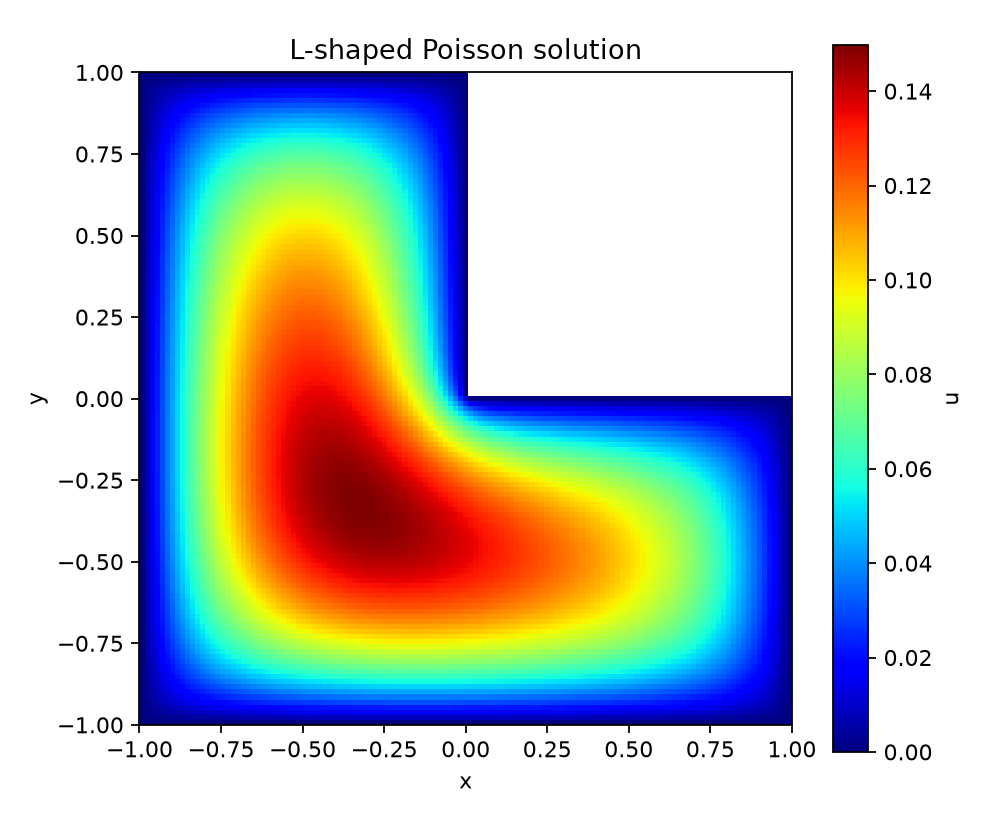
In this example, an L-shaped domain is created by subtracting the square [0,1] × [0,1] from the outer square [-1,1] × [-1,1]. The geometry is evaluated on a regular grid, and a smoothed mask is generated for visualization and for later use in embedded-domain solving.

import numpy as np
import matplotlib.pyplot as plt

from optixde.geometry.primitives import Rectangle
from optixde.geometry.boolean import Difference

x = np.linspace(-1.0, 1.0, 257)
y = np.linspace(-1.0, 1.0, 257)
X, Y = np.meshgrid(x, y, indexing="xy")
P = np.c_[X.ravel(), Y.ravel()]

geo = Difference(
    Rectangle(-1.0, 1.0, -1.0, 1.0),
    Rectangle(0.0, 1.0, 0.0, 1.0),
)

eps = 2.0 * (x[1] - x[0])
mask = geo.smooth_mask(P, eps=eps).reshape(len(y), len(x))

plt.figure(figsize=(6.2, 5.2))
plt.imshow(
    mask,
    origin="lower",
    cmap="jet",
    extent=[x[0], x[-1], y[0], y[-1]],
)
plt.colorbar(label="mask")
plt.title("Smoothed mask")
plt.tight_layout()
plt.show()

4) Define, solve, and visualize a PDE

Once the computational grid and source term are prepared, solving a PDE in OptiXDE is straightforward.

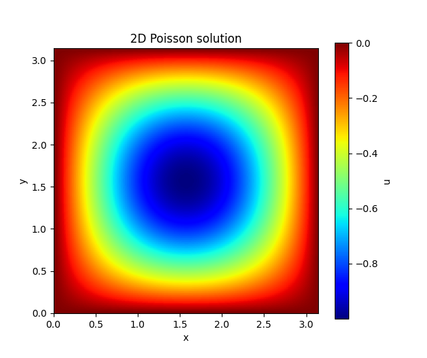
In this example, we consider the 2D Poisson equation on the square domain [0, \pi] \times [0, \pi] with homogeneous Dirichlet boundary conditions, [ -\Delta u = f \quad \text{in } \Omega, ] where the right-hand side is chosen as [ f(x,y)=2\sin(x)\sin(y). ] For this choice, the exact solution is [ u(x,y)=\sin(x)\sin(y), ] which makes the example convenient for verification. After defining the source field on the uniform grid, the Poisson solver is called directly, and the resulting solution is visualized as a color map. This illustrates the basic OptiXDE workflow: define the PDE, solve it on the FFT-compatible grid, and inspect the result immediately.

import numpy as np
import matplotlib.pyplot as plt
from optixde.solvers.base.poisson import poisson2d_solve

Lx = Ly = np.pi
N = 128

dx = Lx / (N + 1)
dy = Ly / (N + 1)
x = np.linspace(dx, Lx - dx, N)
y = np.linspace(dy, Ly - dy, N)
X, Y = np.meshgrid(x, y, indexing="xy")

f = np.zeros((N + 2, N + 2))
f[1:-1, 1:-1] = 2.0 * np.sin(X) * np.sin(Y)

u = poisson2d_solve(f, Lx, Ly, bc="dirichlet", workers=8)

plt.figure(figsize=(6.2, 5.2))
plt.imshow(
    u,
    cmap="jet",
    origin="lower",
    extent=[0, Lx, 0, Ly],
)
plt.colorbar(label="u")
plt.title("2D Poisson solution")
plt.xlabel("x")
plt.ylabel("y")
plt.show()

5) Understand grid and boundary-condition conventions

Two-dimensional fields in OptiXDE use shape (Ny, Nx): the first axis is the y direction and the second axis is the x direction. The grid construction depends on the boundary condition because each condition uses a different spectral transform.

Boundary condition	Transform or enforcement	Recommended grid
periodic	FFT	Endpoint excluded
dirichlet	DST on the interior	Physical boundary included
neumann	DCT on the full field	Physical boundary included
robin	Boundary projection / penalty	Physical boundary included

For a periodic domain [0,Lx) × [0,Ly), construct an endpoint-free grid:

x = np.linspace(0.0, Lx, Nx, endpoint=False)
y = np.linspace(0.0, Ly, Ny, endpoint=False)
X, Y = np.meshgrid(x, y, indexing="xy")

For homogeneous Dirichlet conditions, include the physical boundary. The interior values are stored in u[1:-1, 1:-1], while the returned boundary is zero.

x = np.linspace(0.0, Lx, Nx + 2)
y = np.linspace(0.0, Ly, Ny + 2)
X, Y = np.meshgrid(x, y, indexing="xy")
u = np.zeros((Ny + 2, Nx + 2))

For periodic and Neumann Poisson problems, the source must have zero mean. OptiXDE fixes the additive constant of the solution with a zero-mean gauge.

6) Solve a time-dependent PDE

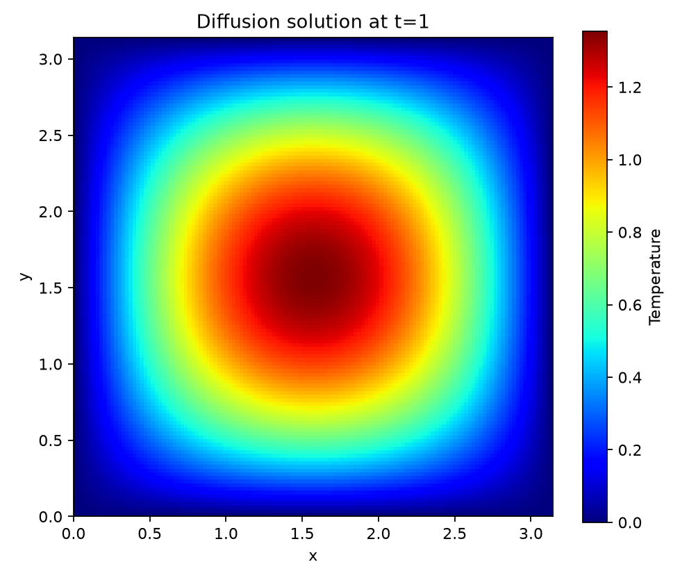
OptiXDE can also advance time-dependent equations. Consider the two-dimensional diffusion equation

\[ \frac{\partial u}{\partial t}=D\Delta u, \]

with homogeneous Dirichlet boundary conditions. Each call to diffusion2d_solve advances the field by one timestep.

import numpy as np
import matplotlib.pyplot as plt
from optixde.solvers import diffusion2d_solve

Lx = Ly = np.pi
N = 128
D = 1.0
dt = 0.05
T = 1.0

dx = Lx / (N + 1)
x = np.linspace(dx, Lx - dx, N)
y = np.linspace(dx, Ly - dx, N)
X, Y = np.meshgrid(x, y, indexing="xy")

u = np.zeros((N + 2, N + 2))
u[1:-1, 1:-1] = 10.0 * np.sin(X) * np.sin(Y)

for _ in range(int(round(T / dt))):
    u = diffusion2d_solve(u, D, Lx, Ly, dt, bc="dirichlet")

plt.figure(figsize=(6.2, 5.2))
plt.imshow(u, cmap="jet", origin="lower", extent=[0, Lx, 0, Ly])
plt.colorbar(label="Temperature")
plt.title(f"Diffusion solution at t={T:g}")
plt.xlabel("x")
plt.ylabel("y")
plt.tight_layout()
plt.show()

7) Solve a PDE on an embedded geometry

The geometry-to-mask workflow can be continued directly into an embedded-domain solve. Here the same L-shaped region is written as a polygon, homogeneous Dirichlet data are assigned to every edge, and

\[ -\Delta u=1 \quad \text{in } \Omega, \qquad u=0 \quad \text{on } \partial\Omega \]

is solved on a Cartesian grid. Install the sparse optional dependency before running this example.

import numpy as np
import matplotlib.pyplot as plt

from optixde.bc.segmented import DirichletBC, EdgeSegment
from optixde.geometry.primitives import Polygon
from optixde.solvers import poisson2d_polygonal_embedded

vertices = np.asarray([
    (0.0, 0.0),
    (1.0, 0.0),
    (1.0, -1.0),
    (-1.0, -1.0),
    (-1.0, 1.0),
    (0.0, 1.0),
])

geo = Polygon(vertices)
bcs = [
    DirichletBC(segment=EdgeSegment(edge_id=i), value=0.0)
    for i in range(len(vertices))
]

u, metadata = poisson2d_polygonal_embedded(
    geometry=geo,
    bcs=bcs,
    source=1.0,
    Nx=129,
    Ny=129,
    return_metadata=True,
)

grid = metadata["grid"]
cmap = plt.cm.jet.copy()
cmap.set_bad("white")

plt.figure(figsize=(6.2, 5.2))
plt.imshow(
    u,
    origin="lower",
    cmap=cmap,
    extent=[grid["x"][0], grid["x"][-1], grid["y"][0], grid["y"][-1]],
)
plt.colorbar(label="u")
plt.title("L-shaped Poisson solution")
plt.xlabel("x")
plt.ylabel("y")
plt.tight_layout()
plt.show()

8) Switch between CPU and GPU backends

NumPy is the default backend. Periodic FFT solvers can use the PyTorch backend on a CPU or CUDA GPU without changing the equation. The following example uses a manufactured periodic Poisson problem with the exact solution sin(2x) cos(3y).

import numpy as np
from optixde.solvers import poisson2d_solve

Lx = Ly = 2.0 * np.pi
N = 128
x = np.linspace(0.0, Lx, N, endpoint=False)
y = np.linspace(0.0, Ly, N, endpoint=False)
X, Y = np.meshgrid(x, y, indexing="xy")
f = 13.0 * np.sin(2.0 * X) * np.cos(3.0 * Y)

u_cpu = poisson2d_solve(
    f, Lx, Ly,
    bc="periodic",
    backend_name="numpy",
)

u_gpu = poisson2d_solve(
    f, Lx, Ly,
    bc="periodic",
    backend_name="torch",
    device="cuda",
)

Use device="cpu" to test the PyTorch path on a machine without CUDA. The Dirichlet and Neumann DCT/DST paths are primarily intended for NumPy arrays.

9) Inspect solver diagnostics

Unified solver entry points support return_info=True. The returned metadata records which numerical path was used and is useful for tests, benchmarks, and GPU checks.

u, info = poisson2d_solve(
    f,
    Lx,
    Ly,
    bc="periodic",
    backend_name="numpy",
    return_info=True,
)

for key in (
    "solver",
    "equation",
    "bc",
    "transform",
    "backend",
    "device",
    "input_shape",
    "output_shape",
):
    print(f"{key}: {info[key]}")

Typical transform values include fft, dst, dct, and robin_penalty. Equation-specific metadata may also report the timestep, diffusivity, wave speed, viscosity, or other solver parameters.

10) Explore more equations

The same public solver namespace provides elliptic, evolution, nonlinear, wave, and flow equations.

Equation or topic	Main public entry points	Guide
Poisson and Helmholtz	poisson2d_solve, helmholtz2d_solve	Elliptic solvers
Diffusion and wave	diffusion2d_solve, wave2d_solve	Evolution equations
Allen--Cahn and Burgers	allen_cahn2d_solve, burgers1d_solve	Evolution equations
Navier--Stokes and cylinder flow	navier_stokes2d_vorticity_solve, cylinder_flow2d_solve	Flow solvers
Schrödinger equations	schrodinger2d_solve, schrodinger1d_cubic_solve	Evolution equations
Polygonal domains	poisson2d_polygonal_embedded, transient_diffusion_polygonal_embedded	Embedded domains

11) Run complete examples

The OptiXDE repository contains complete examples, validation cases, and paper reproduction scripts. After cloning the repository and installing the desired optional dependencies, try these commands:

git clone https://github.com/yangyLab/OptiXDE.git
cd OptiXDE
pip install -e ".[plot,sparse]"

# Minimal time-dependent diffusion example
python examples/base/diffusion_dirichlet_minimal_demo.py

# Embedded L-shaped Poisson example
python examples/base/poisson_lshape_deepxde_benchmark.py \
  --n 129 \
  --output examples/artifacts/lshape_quickstart.png

# PyTorch backend smoke test; use --device cuda on a CUDA runtime
python examples/benchmarks/colab_torch_gpu_smoke.py --device cpu --n 64

Examples do not save figures by default unless an output path is supplied. Use --output or --output-dir to keep generated figures, CSV files, and tables. See the Benchmarks page for larger verification and performance studies.