Method

1. Core idea

OptiXDE treats a differential equation as an operator acting on a field sampled on a uniform Cartesian grid. When the linear spatial operator is diagonal in a Fourier, sine, or cosine basis, differentiation and time evolution reduce to independent operations on spectral modes.

For

\[ \frac{\partial u}{\partial t}=\mathcal{L}u, \]

let \(\lambda(\mathbf{k})\) be the spectral symbol of \(\mathcal{L}\). A linear time step is

\[ \widehat{u}^{\,n+1}(\mathbf{k}) = \underbrace{ \exp\!\left[\lambda(\mathbf{k})\Delta t\right] }_{G(\mathbf{k},\Delta t)} \widehat{u}^{\,n}(\mathbf{k}), \]

or, in physical space,

\[ u^{n+1} = \mathcal{F}^{-1} \left[ G(\mathbf{k},\Delta t)\, \mathcal{F}[u^n] \right]. \]

This transform--propagate--inverse-transform loop is the main computational pattern in OptiXDE. It replaces stiffness-matrix assembly with FFTs and pointwise spectral multiplication for the rectangular spectral solvers.

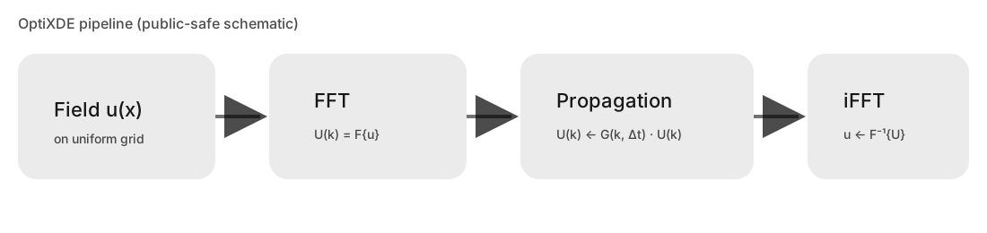
Role of OptiXDE

Fourier propagation itself is classical. OptiXDE combines it with reusable backends, cached operators, boundary transforms, nonlinear splitting, geometry tools, diagnostics, and post-processing in one consistent solver interface.

2. Discrete spectral grid

For a periodic rectangle \(\widetilde{\Omega}=[0,L_x)\times[0,L_y)\), the field is stored with shape (Ny, Nx) on

\[ x_j=\frac{jL_x}{N_x}, \qquad y_\ell=\frac{\ell L_y}{N_y}. \]

The FFT-ordered angular wave numbers are

\[ k_x=2\pi\,\mathrm{fftfreq}(N_x,L_x/N_x), \qquad k_y=2\pi\,\mathrm{fftfreq}(N_y,L_y/N_y), \]

and OptiXDE caches the two-dimensional grids and

\[ K^2=k_x^2+k_y^2. \]

The first array axis is \(y\), and the second is \(x\). NumPy, CuPy, and PyTorch backends use the same layout. Cache keys include grid size, domain length, dtype, and device, preventing incompatible frequency grids or propagators from being reused.

3. Linear propagation and inversion

The diffusion equation illustrates the basic construction:

\[ \frac{\partial u}{\partial t}=D\Delta u. \]

Fourier transformation gives

\[ \frac{\partial\widehat u}{\partial t} = -DK^2\widehat u, \]

so each mode can be integrated analytically:

\[ \widehat u^{\,n+1} = \exp(-DK^2\Delta t)\widehat u^{\,n}. \]

Because the multiplier has magnitude no greater than one for \(D,\Delta t\ge0\), the constant-coefficient linear diffusion step is non-expansive and has no explicit diffusion stability limit.

Other linear equations use the same structure with a different diagonal operator:

Equation	Spectral treatment
Diffusion \(u_t=D\Delta u\)	\(\exp(-DK^2\Delta t)\)
Poisson \(-\Delta u=f\)	\(\widehat u=\widehat f/K^2\), with the zero mode fixed
Shifted Helmholtz \((-\Delta+k_0^2)u=f\)	\(\widehat u=\widehat f/(K^2+k_0^2)\)
Wave \(u_{tt}=c^2\Delta u\)	exact modal oscillator update for displacement and velocity
Free Schrödinger \(\psi_t=ia\Delta\psi\)	\(\exp(-iaK^2\Delta t)\)

For periodic Poisson and Neumann Poisson problems, the Laplacian has a constant nullspace. OptiXDE can subtract the mean of \(f\) to enforce compatibility and sets the solution zero mode to fix the additive gauge.

For periodic diffusion with a source, OptiXDE provides an ETD1 update using

\[ \varphi_1(z)=\frac{\exp(z)-1}{z}, \qquad \varphi_1(0)=1, \]

with a stable small-\(z\) approximation. The source is sampled at the midpoint of the step.

4. Nonlinear equations and splitting

For

\[ u_t=\mathcal{L}u+\mathcal{N}(u), \]

OptiXDE propagates the constant-coefficient linear part in spectral space and evaluates nonlinear products in physical space. This pseudo-spectral approach avoids forming convolution sums explicitly:

\[ u=\mathcal{F}^{-1}[\widehat u], \qquad \widehat{\mathcal{N}} = \mathcal{F}[\mathcal{N}(u)]. \]

The library provides first-order Lie splitting and symmetric second-order Strang splitting:

\[ \text{Lie:}\quad \Phi_N(\Delta t)\Phi_L(\Delta t), \]

\[ \text{Strang:}\quad \Phi_L(\Delta t/2) \Phi_N(\Delta t) \Phi_L(\Delta t/2). \]

Representative implementations are:

Solver	Linear part	Physical-space or nonlinear part
Allen--Cahn	spectral diffusion	exact pointwise reaction \(u-u^3\)
Periodic Burgers	exact Fourier diffusion half-steps	conservative convection with Euler or midpoint RK2
Cubic Schrödinger	Fourier dispersion half-steps	exact local nonlinear phase
Periodic Navier--Stokes	Fourier viscosity and Poisson inversion	conservative vorticity flux with Euler or midpoint RK2

Quadratic nonlinearities can use the two-thirds de-aliasing rule. This removes unresolved high-frequency content produced by physical-space multiplication.

Linear stability is not complete stability

An exact linear propagator does not remove timestep restrictions introduced by explicit nonlinear terms, operator splitting, embedded-boundary updates, or finite-difference substeps. Nonlinear calculations still require timestep and resolution studies.

5. Boundary conditions on rectangles

For coordinate-aligned rectangular domains, OptiXDE selects a transform whose basis satisfies the homogeneous boundary condition:

Boundary condition	Numerical treatment
Periodic	FFT on an endpoint-excluded grid
Homogeneous Dirichlet	DST on the interior of a full endpoint-inclusive grid
Homogeneous Neumann	DCT on a full endpoint-inclusive grid
Robin	spectral prediction or preconditioning plus local boundary projection

The DST path returns zero boundary values. The DCT path includes the constant mode and therefore exposes the Poisson compatibility and gauge controls.

Nonhomogeneous Dirichlet Poisson data can be treated by a lifting

\[ u=v+T_b, \qquad v|_{\partial\Omega}=0, \]

where a Coons patch \(T_b\) matches the four boundary curves and the homogeneous correction \(v\) is solved with the DST kernel.

For rectangular Robin data,

\[ \alpha u+\beta\partial_nu=g, \]

the current implementation uses one-sided finite-difference projection on each side. Poisson combines this projection with a preconditioned iteration; diffusion applies a spectral prediction followed by local boundary projections. Homogeneous Dirichlet or Neumann limits are routed to DST or DCT when possible.

6. Geometry and embedded domains

Signed-distance convention

The geometry package uses the positive-inside convention:

\[ d(\mathbf{x})>0\ \text{inside }\Omega,\qquad d(\mathbf{x})=0\ \text{on }\partial\Omega,\qquad d(\mathbf{x})<0\ \text{outside }\Omega. \]

Accordingly,

\[ d_{A\cup B}=\max(d_A,d_B),\qquad d_{A\cap B}=\min(d_A,d_B),\qquad d_{A\setminus B}=\min(d_A,-d_B). \]

Rectangle, disk, sphere, and polygon primitives can therefore be combined without a body-fitted mesh.

Masks and boundary bands

The hard interior mask is

\[ m_\Omega^0=\mathbf{1}_{d\ge0}. \]

A smooth mask and boundary weight are also available:

\[ m_\Omega = \frac12 \left[ 1+\tanh\!\left(\frac{d}{\varepsilon}\right) \right], \]

\[ w_\Gamma = \frac{1}{2\varepsilon} \operatorname{sech}^2\!\left(\frac{d}{\varepsilon}\right). \]

The smoothing thickness \(\varepsilon\) is expressed in physical units and is typically chosen on the order of one to three grid spacings. Smoothing reduces Gibbs-type oscillation from a discontinuous mask, but introduces a finite interface layer that must be considered in refinement studies.

Current embedded-domain paths

The general operator-level form is

\[ u^{n+1} = \mathcal{E}_{\Omega,\Gamma} \left( \mathcal{T}_G[u^n] \right), \]

where \(\mathcal{T}_G\) is a propagation step and \(\mathcal{E}_{\Omega,\Gamma}\) applies geometry or boundary constraints in physical space.

The current library exposes two practical routes:

1. hard masks, smooth masks, and boundary weights for penalty-style spectral workflows and custom solvers;
2. segmented polygon solvers that rasterize Dirichlet, Neumann, and Robin data on Cartesian grids.

The segmented steady Poisson solver assembles a sparse masked-grid system. Transient polygon diffusion and wave utilities use explicit masked finite differences. These solvers share OptiXDE's geometry and boundary abstractions, but their current numerical kernel is not a pure FFT propagator.

7. Implementation and complexity

For a periodic linear problem, preprocessing constructs the grid and retrieves or creates the frequency arrays and propagation multiplier. Each subsequent step performs:

forward transform
→ pointwise spectral propagation
→ inverse transform
→ optional nonlinear, boundary, geometry, or diagnostic operations

Static arrays remain on the selected device. Backend caches reuse frequency grids, while PropagatorCache reuses exponential and inverse-\(K^2\) multipliers.

For \(N\) grid points, an FFT-based propagation step requires

\[ \mathcal{O}(N\log N) \]

work and

\[ \mathcal{O}(N) \]

memory. Pointwise propagation, nonlinear products, masks, and local boundary corrections are \(\mathcal{O}(N)\) and naturally parallel.

This complexity applies to the rectangular FFT solvers. The segmented Poisson solver additionally solves a sparse system, and the inlet/outlet cylinder-flow solver uses a cached sparse pressure factorization.

8. Accuracy and scope

Smooth periodic problems can exhibit spectral spatial convergence. In practice, accuracy may instead be limited by nonsmooth data, geometric corners, unresolved nonlinear scales, mask thickness, boundary projection, or floating-point precision.

The spectral core is best suited to uniform Cartesian grids and constant-coefficient operators diagonalizable by FFT, DST, or DCT. Variable coefficients and irregular interfaces require splitting, correction, or an alternative discretization. OptiXDE exposes these paths explicitly rather than presenting them as one universally exact propagator.

For function signatures, backend options, and return contracts, see the API reference.