Benchmarks

This page reports reproducible results generated by the current OptiXDE examples. The emphasis is on accuracy, convergence behavior, physical diagnostics, and difficult geometry. Values are taken from saved result files or the convergence output of the linked benchmark scripts; no placeholder timing or error data are used.

Benchmark summary

Problem	Discretization	Reference or diagnostic	Main observation
Poisson on an L-shaped domain	FFT-compatible embedding with smoothed penalization	Singular harmonic reference	Error is localized near the re-entrant corner and embedded interface
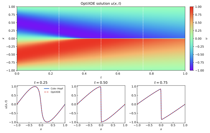
1D viscous Burgers	FFT splitting with odd periodic extension	Cole--Hopf quadrature	Approximately second-order temporal convergence
2D Allen--Cahn	Spectral diffusion and exact reaction, Strang splitting	Independent Fourier ETDRK4	Second-order temporal convergence and monotone free-energy decay
1D cubic Schrödinger	Split-step Fourier method	Fine-grid Fourier RK4	Near second-order behavior before the spatial/reference error floor
2D Navier--Stokes	Periodic vorticity--streamfunction FFT splitting	Taylor--Green analytical decay	Vorticity, divergence, and enstrophy agree to near machine precision

Interpreting the tables

Rates are computed between successive timestep or grid refinements. A reduced rate at the finest level does not necessarily indicate instability: once temporal error is small, spatial discretization and reference-solution error can dominate.

Poisson problem on an L-shaped domain

The physical domain is

\[ \Omega=(-1,1)^2\setminus([0,1]\times[-1,0]), \]

with a re-entrant corner of angle \(3\pi/2\). The analytical reference is the singular harmonic field

\[ u_{\mathrm{ex}}(r,\theta) =r^{2/3}\sin(2\theta/3). \]

The domain is embedded in a periodic Cartesian box. Dirichlet data are imposed through a smoothed Brinkman-type penalty layer with \(\eta=0.003h^2\) and \(\varepsilon=\max(0.03,2.5h)\).

Download the vector PDF

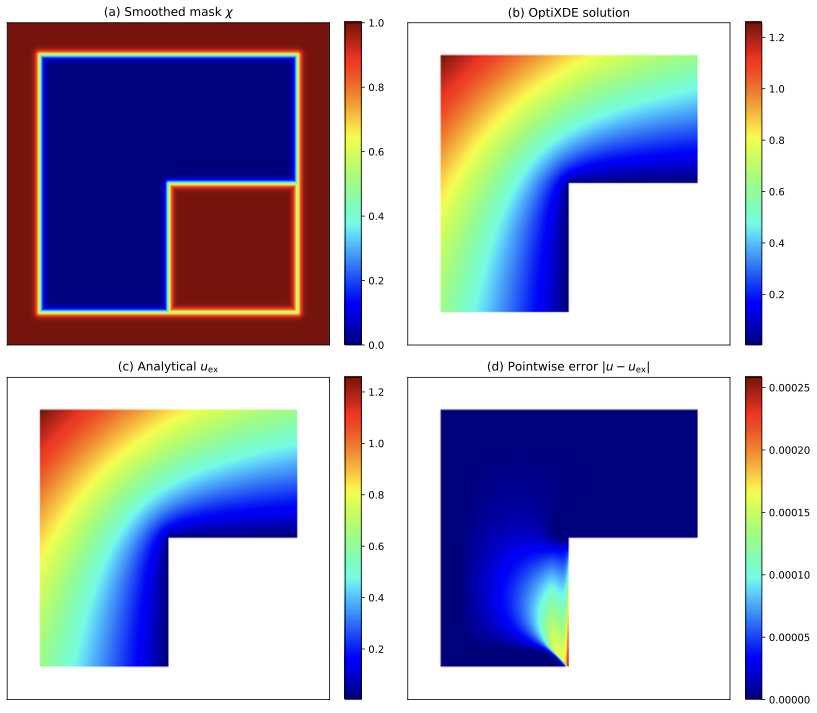
Global error

Grid	\(e_{L^2}(\Omega)\)	Rate
\(256^2\)	\(1.571034\times10^{-3}\)	--
\(384^2\)	\(1.989538\times10^{-4}\)	5.096
\(512^2\)	\(3.145243\times10^{-5}\)	6.412
\(768^2\)	\(1.000724\times10^{-5}\)	2.824

Smooth-interior error

The interior metric excludes a neighborhood of the singular corner and a thin embedded-boundary layer.

Grid	\(e_{L^2}(\Omega_{\mathrm{in}})\)	Rate
\(256^2\)	\(1.705635\times10^{-3}\)	--
\(384^2\)	\(2.139415\times10^{-4}\)	5.120
\(512^2\)	\(2.867095\times10^{-5}\)	6.986
\(768^2\)	\(2.246577\times10^{-6}\)	6.280

The global norm eventually reflects the corner singularity and finite penalty layer, whereas the field away from both regions retains rapid, spectral-like refinement behavior.

Script: poisson_lshape_penalty_benchmark.py

Viscous Burgers equation

The benchmark solves

\[ u_t+u\,u_x=\nu u_{xx}, \qquad \nu=\frac{0.01}{\pi}, \]

on \([-1,1]\) with homogeneous Dirichlet data. The endpoint-inclusive physical solution uses \(N_x=1024\), while an odd extension produces a 2048-point periodic field for FFT propagation. The nonlinear conservative flux is de-aliased with the two-thirds rule, and the reference solution is evaluated from the Cole--Hopf representation using 8192 quadrature points.

Download the solution PDF

\(\Delta t\)	\(e_{L^2}(T)\)	\(e_\infty(T)\)	Rate
\(1.00\times10^{-3}\)	\(4.450652\times10^{-5}\)	\(2.836634\times10^{-4}\)	--
\(5.00\times10^{-4}\)	\(1.123266\times10^{-5}\)	\(7.035812\times10^{-5}\)	1.986
\(2.50\times10^{-4}\)	\(2.821009\times10^{-6}\)	\(1.712867\times10^{-5}\)	1.993
\(1.25\times10^{-4}\)	\(7.135400\times10^{-7}\)	\(4.065077\times10^{-6}\)	1.983

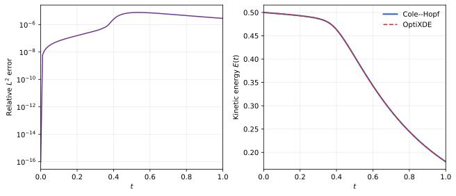
The measured rate is consistently close to two, matching the midpoint nonlinear update within the symmetric diffusion splitting. The maximum boundary residual is \(5.10\times10^{-14}\), and the kinetic-energy history is monotone to reported precision.

Download the diagnostics PDF

Script: burgers_1d_deepxde_benchmark.py

Two-dimensional Allen--Cahn equation

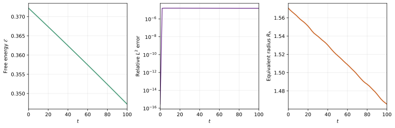
The phase-field benchmark advances

\[ u_t=\varepsilon^2\Delta u+u-u^3, \qquad \varepsilon=0.04, \]

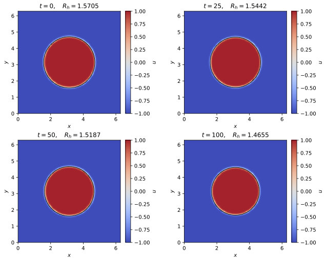
on a \(256^2\) periodic grid to \(T=100\). Spectral diffusion is combined with the exact pointwise reaction flow by Strang splitting. The independent reference uses Fourier ETDRK4 on a \(512^2\) grid with \(\Delta t_{\mathrm{ref}}=0.05\).

Download the field-evolution PDF

\(\Delta t\)	\(e_{L^2}(T)\)	Rate	\(\mathcal{E}(T)\)	\(R_h(T)\)
\(2.0\times10^{-1}\)	\(2.452780\times10^{-4}\)	--	0.34722423	1.46550466
\(1.0\times10^{-1}\)	\(6.167643\times10^{-5}\)	1.992	0.34722108	1.46550606
\(5.0\times10^{-2}\)	\(1.544310\times10^{-5}\)	1.998	0.34722081	1.46550643
\(2.5\times10^{-2}\)	\(3.862123\times10^{-6}\)	1.999	0.34722078	1.46550653

The timestep study shows second-order convergence. The free energy decreases from 0.37220609 to approximately 0.3472208 with no detected monotonicity violation. The equivalent radius decreases from 1.57049 to 1.46551, making the curvature-driven interface motion visible over the chosen time interval.

Download the diagnostics PDF

Script: allen_cahn_raissi_3_2_1_reproduction.py

Cubic Schrödinger equation

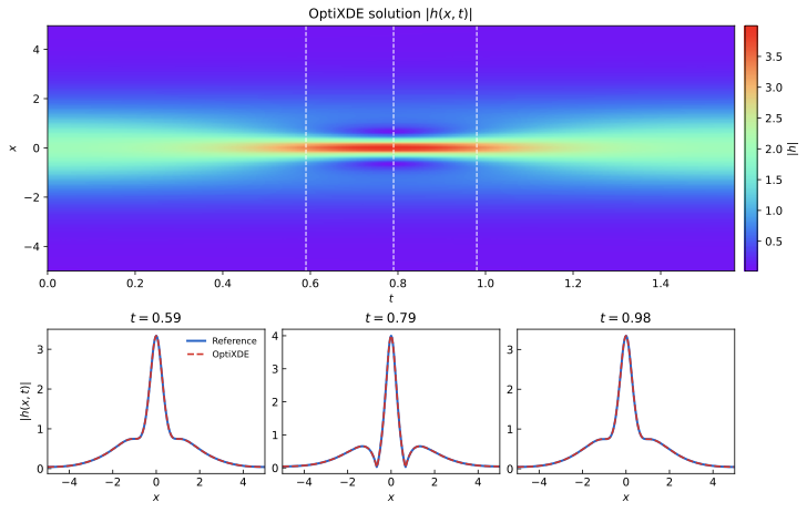
The one-dimensional focusing cubic nonlinear Schrödinger equation is solved with a periodic split-step Fourier method. The benchmark uses \(N_x=256\); the independent reference uses 2048 Fourier modes and \(\Delta t_{\mathrm{ref}}=6.25\times10^{-6}\).

Download the solution PDF

\(\Delta t\)	\(e_{\max}\)	Rate	Mass drift	Hamiltonian drift
\(2.0\times10^{-3}\)	\(3.439933\times10^{-4}\)	--	\(9.19\times10^{-14}\)	\(7.15\times10^{-8}\)
\(1.0\times10^{-3}\)	\(8.703352\times10^{-5}\)	1.983	\(6.62\times10^{-14}\)	\(2.92\times10^{-8}\)
\(5.0\times10^{-4}\)	\(2.710324\times10^{-5}\)	1.683	\(3.40\times10^{-13}\)	\(1.94\times10^{-10}\)
\(2.5\times10^{-4}\)	\(1.803587\times10^{-5}\)	0.588	\(8.37\times10^{-13}\)	\(4.99\times10^{-11}\)

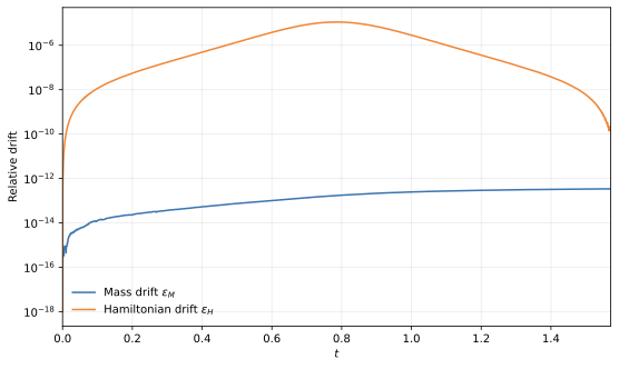
The two coarser steps exhibit the expected second-order splitting behavior. At finer steps, the rate decreases as temporal error approaches the spatial/reference floor. Mass remains conserved to approximately \(10^{-12}\) or better, while the Hamiltonian drift decreases to \(5.0\times10^{-11}\).

Download the invariant-diagnostics PDF

Script: schrodinger_raissi_3_1_1_reproduction.py

Two-dimensional Navier--Stokes equation

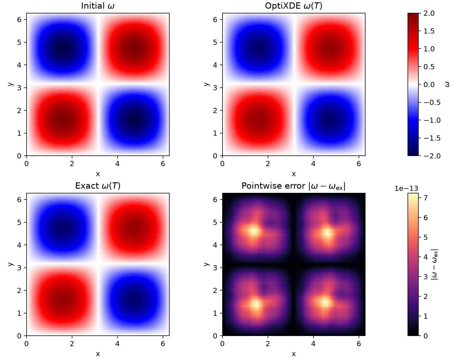
The Taylor--Green vortex verifies the periodic incompressible vorticity--streamfunction solver. On \([0,2\pi)^2\), the initial vorticity is

\[ \omega(x,y,0)=2\sin x\sin y, \]

and the exact viscous decay is

\[ \omega_{\mathrm{ex}}(x,y,t) = 2\exp(-2\nu t)\sin x\sin y. \]

The corresponding velocity remains divergence free, and the enstrophy

\[ \mathcal{Z}(t) = \frac12\int_\Omega\omega^2\,d\Omega \]

decays as \(\mathcal{Z}(t)=\mathcal{Z}(0)\exp(-4\nu t)\).

The reported run uses a \(128^2\) periodic grid, \(\nu=0.05\), \(\Delta t=10^{-3}\), and \(T=1\). OptiXDE applies exact Fourier diffusion half-steps, midpoint RK2 for the conservative vorticity flux, and two-thirds de-aliasing.

Download the vector PDF

Diagnostic	Value
Relative \(L^2\) vorticity error	\(2.906326\times10^{-13}\)
Maximum pointwise vorticity error	\(7.236434\times10^{-13}\)
Maximum \(\lvert\nabla\cdot\mathbf{u}\rvert\)	\(2.231548\times10^{-14}\)
RMS velocity divergence	\(5.840040\times10^{-15}\)
Initial enstrophy	\(1.973920880218\times10^{1}\)
Final enstrophy	\(1.616109728778\times10^{1}\)
Exact final enstrophy	\(1.616109728777\times10^{1}\)
Relative enstrophy error	\(5.680439\times10^{-13}\)
Maximum final speed	\(9.048374\times10^{-1}\)

The Taylor--Green field is a single resolved Fourier-mode configuration whose nonlinear vorticity advection vanishes analytically. The near-machine-precision result therefore verifies spectral differentiation, velocity reconstruction, viscous propagation, and incompressibility for this special solution. It should not be interpreted as the expected error for a broadband turbulent flow.

Script: navier_stokes_taylor_green.py

Reproducibility notes

• Tables report the values written by the corresponding scripts.
• PDF files are the original vector outputs; PNG files are web previews rendered from those PDFs.
• Errors should be compared only when the grid, time interval, reference solution, and norm definition agree.
• Performance numbers are intentionally omitted until runs record hardware, backend, precision, warm-up policy, and timing methodology. This avoids publishing machine-dependent placeholder values.